Selecting a peerless component requires a rigorous evaluation of noise figure, gain, linearity, and process technology to ensure the receiver maintains maximum sensitivity. Imagine you are designing a high-performance wireless system, but the incoming signal is so weak it gets buried under the internal thermal noise of your hardware. This frustrating loss of data integrity can jeopardize entire projects, leading to signal degradation and poor system range. Integrating a high-quality Low Noise Amplifier serves as the primary solution by boosting weak signals at the very start of the RF front-end while contributing virtually no noise of its own.
What is Cascaded Noise Figure in a Low Noise Amplifier?
Cascaded noise figure refers to the total noise contribution of a multi-stage system where the performance of the first component determines the overall sensitivity. When you integrate a Low Noise Amplifier into a system, the Friis formula dictates that the noise of the first stage is the most critical factor. This means any noise introduced later in the signal chain is suppressed by the gain of the preceding stages.
The Impact of Multi-Stage Architecture
In a cascaded system, every additional component adds its own noise to the signal path. If the initial stage does not provide enough gain or has a high noise figure, the entire receiver’s performance will suffer regardless of how “quiet” the later stages are.
Here is the deal:
You must calculate the system noise budget early in the design phase.
- First stage noise is additive.
- Second stage noise is divided by first stage gain.
- Third stage noise becomes almost negligible if prior gain is high.
Why the First Stage Dominates Performance
The first stage is the gatekeeper of your signal-to-noise ratio. By selecting a component with an ultra-low noise figure and sufficient gain, you effectively “mask” the noise of lossy components like mixers or filters that follow.
Think about it this way:
If your first stage gain is 20dB, the noise of the second stage is reduced by a factor of 100. This is why the primary LNA is the most important purchase for your RF front end.
Key Takeaway: Prioritizing the noise figure of the very first amplifier in your chain is the most cost-effective way to improve total system sensitivity.
| Parameter | Impact on System | Priority |
|---|---|---|
| First Stage NF | Direct increase in system noise | High |
| First Stage Gain | Suppresses downstream noise | High |
| Second Stage NF | Minimal impact if first stage gain is high | Low |
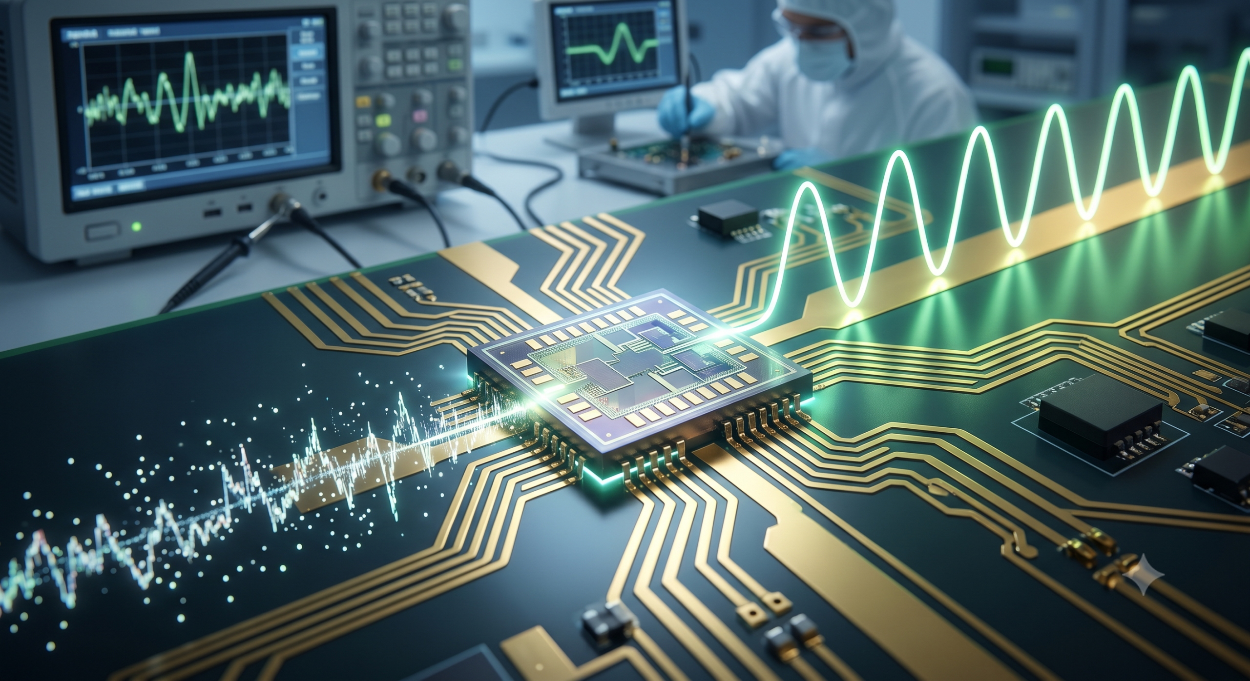
The following data illustrates how gain in the early stages preserves the integrity of the original signal throughout the receiver chain.
How does Gain affect your Low Noise Amplifier choice?
Gain determines the degree of amplification applied to the input signal to ensure it stays well above the noise floor of subsequent components. Choosing a Low Noise Amplifier with the right gain profile is a balancing act between sensitivity and system headroom. You need enough gain to overcome downstream losses but not so much that you drive the next stage into distortion.
Balancing Signal Strength and Noise
While high gain is generally desirable for noise suppression, it can come at a cost. Excessive gain can amplify unwanted background interference just as much as the desired signal, potentially reducing the usable signal-to-noise ratio in crowded environments.
But wait, there’s more:
- Higher gain improves cascaded noise figures.
- Lower gain preserves linearity in strong-signal areas.
- Variable gain options provide flexibility for dynamic environments.
Potential for Downstream Saturation
If your LNA provides too much power, it may saturate the mixers or analog-to-digital converters that follow it. This leads to clipping and the generation of harmonics that can corrupt your data.
You might be wondering:
How do I find the “sweet spot”? You should analyze the compression points of every component in your signal chain to ensure the LNA output never exceeds their input limits.
Key Takeaway: Select a gain level that provides at least 10-15dB more than the noise figure of the following stage to ensure optimal system performance.
| Gain Level | Advantage | Risk |
|---|---|---|
| Low (<15dB) | High Linearity | Poor Noise Suppression |
| Medium (15-25dB) | Balanced Performance | Moderate Power Use |
| High (>25dB) | Excellent Sensitivity | Risk of Saturation |
Effective gain management ensures that the signal remains clean and detectable even in the presence of significant path loss.
Why is Bandwidth critical for a Low Noise Amplifier?
Bandwidth defines the range of frequencies over which the amplifier can operate while maintaining its specified noise and gain performance. When selecting a Low Noise Amplifier, you must ensure the device supports your entire operational spectrum without significant roll-off. A mismatch in bandwidth can lead to signal attenuation at the edges of your frequency band.
Operational Frequency Range Requirements
Modern communication systems often operate across multiple bands or utilize wideband modulation schemes. If your LNA is too narrowband, it will act as a filter, potentially cutting off vital parts of your signal or introducing phase distortion.
Here is the deal:
- Narrowband LNAs often offer the lowest noise figures.
- Wideband LNAs provide versatility for multi-protocol systems.
- Ultra-wideband designs require careful impedance matching.
Maintaining Flatness Across the Band
Gain flatness is just as important as the absolute bandwidth. If the gain varies significantly across your frequency range, the system will experience inconsistent performance, making calibration difficult and potentially causing data errors.
It gets better:
High-quality designs use internal compensation to keep gain variations within +/- 0.5dB across the target frequency. This ensures that every channel in your system receives equal amplification.
Key Takeaway: Always verify that the LNA bandwidth exceeds your signal bandwidth to prevent edge-of-band degradation and ensure uniform gain.
| Frequency Type | Application | Primary Benefit |
|---|---|---|
| Narrowband | Satellite, GPS | Maximum Sensitivity |
| Wideband | Electronic Warfare | Spectrum Coverage |
| Multi-band | Cellular Base Stations | Hardware Consolidation |
The relationship between bandwidth and gain flatness is a fundamental pillar of consistent RF system design and reliable data transmission.
How does Linearity impact Low Noise Amplifier performance?
Linearity refers to the amplifier’s ability to boost a signal without adding distortion or creating new, unwanted frequency components. In a Low Noise Amplifier, high linearity is essential when the receiver must operate in the presence of strong interfering signals. If the LNA is non-linear, these “blockers” can cause intermodulation distortion that masks the weak signal you are trying to detect.
Understanding the 1dB Compression Point
The 1dB compression point (P1dB) is a measure of the power level where the amplifier starts to saturate. As you approach this limit, the gain begins to decrease, and the output is no longer a linear representation of the input.
But wait, there’s more:
- P1dB indicates the maximum usable output power.
- Higher P1dB allows for better handling of strong signals.
- It is a critical spec for systems near high-power transmitters.
The Importance of Third-Order Intercept Point
The Third-Order Intercept Point (IP3) is a theoretical value used to predict the level of intermodulation distortion. A higher IP3 means the amplifier can handle multiple strong signals simultaneously without creating interference that falls within your desired band.
Check this out:
For every 1dB increase in input power, third-order distortion products increase by 3dB. This is why a high IP3 is the gold standard for high-performance receiver design.
Key Takeaway: Choose an LNA with an IP3 at least 10dB higher than your strongest expected interference signal to prevent receiver desensitization.
| Metric | Definition | Importance |
|---|---|---|
| P1dB | Power where gain drops by 1dB | Signal Headroom |
| OIP3 | Output Third-Order Intercept | Distortion Resistance |
| Harmonics | Multiples of input frequency | Spectral Purity |
Analyzing these linearity metrics helps engineers prevent signal “crushing” in environments where the RF spectrum is heavily congested.
What defines the Dynamic Range of a Low Noise Amplifier?
Dynamic range is the spread between the smallest detectable signal and the largest signal the amplifier can handle without distortion. A Low Noise Amplifier with a wide dynamic range is necessary for applications like radar or mobile communications where signal levels vary wildly. This ensures that you can hear a faint whisper even when a “loud” transmitter is nearby.
Determining the Lower Sensitivity Limit
The bottom of the dynamic range is set by the noise floor, which is determined by the noise figure and the bandwidth. To detect ultra-weak signals, you must minimize this floor through superior thermal noise management.
Here is the deal:
- Lower noise figures expand the dynamic range downward.
- Reducing bandwidth also lowers the noise floor.
- Temperature control can further improve sensitivity.
Managing Large Signal Handling Capacity
The top end of the dynamic range is limited by the saturation points we discussed in the linearity section. An amplifier that can handle large signals without saturating allows the system to remain functional in “high-clutter” environments.
You should know:
A “spurious-free” dynamic range is often the most important metric. This measures the range where the signal is above the noise floor but all distortion products remain below it.
Key Takeaway: Wide dynamic range is the best defense against signal fading and interference, ensuring reliable communication across diverse environments.
| Factor | Effect on Dynamic Range | Solution |
|---|---|---|
| Noise Figure | Sets the bottom limit | Use high-quality pHEMT |
| P1dB | Sets the top limit | Increase bias current |
| Bandwidth | Influences noise floor | Optimize for target band |
A robust dynamic range allows your hardware to adapt to real-world conditions where signal strength is rarely constant.
How do Process and Cost shape Low Noise Amplifier selection?
Process technology refers to the semiconductor material and manufacturing method used to create the Low Noise Amplifier. Different processes, such as GaAs, GaN, or CMOS, offer varying levels of performance, power handling, and price points. You must weigh the high performance of exotic materials against the lower cost and higher integration of silicon-based solutions.
Semiconductor Material Advancements
GaAs (Gallium Arsenide) pHEMT technology is currently the standard for high-performance LNAs because it offers an exceptionally low noise figure at high frequencies. However, newer processes like GaN (Gallium Nitride) are gaining ground due to their ability to handle much higher input power without damage.
But wait, there’s more:
- GaAs offers the best noise-to-cost ratio.
- CMOS allows for massive integration and low price.
- GaN provides superior survivability and power density.
Evaluating Total Cost of Ownership
The “cheapest” chip might end up being the most expensive if it requires complex external circuitry or fails prematurely. You should consider the cost of peripheral components, PCB area, and the engineering time required for matching and stabilization.
Here is the truth:
An integrated MMIC (Monolithic Microwave Integrated Circuit) might have a higher unit cost than discrete transistors, but it often reduces total system cost by simplifying the design and assembly process.
Key Takeaway: Match the semiconductor process to your specific frequency and power requirements to avoid overpaying for unnecessary performance.
| Process | Typical NF | Cost | Use Case |
|---|---|---|---|
| Silicon (CMOS) | 1.5 – 3.0 dB | Low | Consumer Electronics |
| GaAs pHEMT | 0.5 – 1.2 dB | Medium | Telecom & Satcom |
| GaN | 1.0 – 2.0 dB | High | Military & Radar |
The choice of semiconductor material fundamentally dictates the physical and electrical boundaries of your final amplifier design.
Why manage Bias Voltage in a Low Noise Amplifier?
Bias voltage is the DC power supplied to the amplifier to set its operating point and ensure the internal transistors function correctly. When working with a Low Noise Amplifier, the stability and level of this voltage directly influence gain, noise figure, and linearity. Even small fluctuations in the supply line can introduce noise or cause the amplifier’s performance to drift over time.
Supply Voltage Influence on Headroom
The amount of voltage you provide often dictates the maximum signal swing the amplifier can handle. If the voltage is too low, the device will saturate early, severely limiting your linearity and dynamic range.
Check this out:
- Higher bias voltage generally increases P1dB.
- Lower voltage is preferred for battery-powered devices.
- Standard ranges are often 3V to 5V for most MMICs.
Regulation for Consistent Performance
Using a high-quality, low-noise linear regulator (LDO) is essential for powering an LNA. Switching regulators can introduce ripples and electromagnetic interference (EMI) that bypass the amplifier’s noise suppression and degrade the signal.
Here is the deal:
You should always place decoupling capacitors as close to the bias pins as possible. This filters out high-frequency noise and provides a local reservoir of energy for quick signal transitions.
Key Takeaway: Invest in a clean, regulated power supply to ensure your LNA maintains its rated noise figure and prevents performance drift.
| Supply Issue | Impact on LNA | Prevention |
|---|---|---|
| Voltage Ripple | Increases output noise | Use LDO regulators |
| Under-voltage | Loss of gain and linearity | Monitor supply levels |
| Over-voltage | Permanent device damage | Use Zener protection |
Proper biasing is the foundation of a stable amplifier, ensuring that the hardware operates exactly as the datasheet promises.
How does Current influence Low Noise Amplifier efficiency?
Current consumption in an LNA is primarily driven by the quiescent current, which is the electricity used when no signal is present. While you might want to minimize current to save power, the current level is often tied directly to the device’s linearity. A Low Noise Amplifier biased with more current can typically handle larger signals without distorting.
The Role of Quiescent Current
The quiescent current (Idq) determines the “class” of operation for the amplifier. In many high-performance LNAs, increasing the current can slightly improve the noise figure and significantly boost the IP3.
But wait, there’s more:
- Low current is ideal for remote sensors.
- High current is necessary for base stations.
- Some LNAs allow you to adjust the current with an external resistor.
Thermal Management and Power Dissipation
Every milliamp of current generates heat within the semiconductor die. If you do not manage this heat through proper PCB grounding and thermal vias, the LNA’s noise figure will rise, and its lifespan will decrease.
Consider this:
Heat is the enemy of low noise. For every 10-degree Celsius increase in temperature, the thermal noise floor rises, potentially negating the benefits of a high-end amplifier.
Key Takeaway: Balance your current settings to achieve the required linearity while keeping the device cool enough to maintain a low noise floor.
| Current Setting | Linearity (IP3) | Thermal Load | Battery Life |
|---|---|---|---|
| Low | Moderate | Low | Long |
| Standard | Good | Moderate | Medium |
| High | Excellent | High | Short |
Efficiency in LNA design is not just about saving energy; it is about maintaining a thermal environment conducive to ultra-low noise performance.
Does Impedance Matching matter for a Low Noise Amplifier?
Impedance matching is the process of ensuring that the input and output of the Low Noise Amplifier match the characteristic impedance of the system, usually 50 ohms. Without proper matching, signals will reflect off the amplifier’s ports, causing standing waves (VSWR) and power loss. This can lead to a significant degradation of both gain and noise figure.
Optimizing Input and Output VSWR
The Voltage Standing Wave Ratio (VSWR) is a measure of how well the impedances are matched. A VSWR of 1:1 is a perfect match, while anything above 2:1 indicates significant reflections that can interfere with other components.
Here is the deal:
- Input matching is critical for the noise figure.
- Output matching is critical for power transfer.
- Internal matching simplifies your PCB layout.
Minimizing Return Loss for Signal Integrity
Return loss is the ratio of reflected power to incident power, expressed in decibels. High return loss (indicated by a large negative number, like -20dB) means very little power is being reflected back to the source.
Look at it this way:
If your input match is poor, the “noise match” of the transistor will also be off. You might have to choose between a match that provides the lowest noise or one that provides the best power transfer.
Key Takeaway: Use high-quality RF capacitors and inductors for external matching networks to avoid adding unnecessary loss and noise to the input path.
| Match Quality | Return Loss | VSWR | Result |
|---|---|---|---|
| Excellent | < -20 dB | < 1.2:1 | Maximum Signal Integrity |
| Good | -15 to -10 dB | 1.5:1 to 2.0:1 | Standard Performance |
| Poor | > -10 dB | > 2.0:1 | Signal Loss / Oscillation |
Precise impedance matching ensures that every bit of energy from the antenna is successfully captured and amplified by the receiver hardware.
Can Stability ensure a reliable Low Noise Amplifier?
Stability ensures that the amplifier does not turn into an oscillator, which would generate its own signals and render the receiver useless. A Low Noise Amplifier must be “unconditionally stable,” meaning it will not oscillate regardless of the impedance it sees at its input or output. This is vital for real-world applications where antennas or cables may not provide a perfect 50-ohm load.
Preventing Unwanted Self-Oscillation
Self-oscillation occurs when there is an internal feedback path that allows the signal to loop back and amplify itself. This usually happens at very high frequencies outside of your target band.
But wait, there’s more:
- Stability factors (K-factor) must be greater than 1.
- Proper grounding is the best defense against oscillation.
- Adding “de-Q-ing” resistors can dampen unstable resonances.
Environmental Factors and Long-Term Reliability
Environmental changes, such as extreme temperature shifts or vibration, can affect the electrical characteristics of the components around the LNA. A stable design accounts for these variables to prevent “intermittent” failures that are difficult to diagnose in the field.
The bottom line:
You should always test your design across the full operating temperature range. What is stable at room temperature might become an oscillator at -40°C or +85°C.
Key Takeaway: Prioritize unconditionally stable LNAs and robust PCB grounding to avoid catastrophic system failures caused by parasitic oscillations.
| Stability Factor | Requirement | Risk if Unmet |
|---|---|---|
| K-Factor | K > 1 | High-frequency oscillation |
| Grounding | Low-inductance path | Feedback loops |
| Decoupling | Broad-spectrum filtering | Power supply noise |
Ensuring stability is the final step in selecting a component that will perform reliably over the entire lifecycle of your RF system.
Conclusion
Selecting a peerless Low Noise Amplifier is a multi-dimensional challenge that requires deep insight into cascaded noise, linearity, and semiconductor processes. By addressing the common pain point of signal-to-noise degradation through careful specification analysis, you can ensure your receiver architecture stands above the competition. We have explored the critical roles of gain, bandwidth, and stability, providing a roadmap for engineering success in any RF environment.
Our vision is to empower RF engineers with the most reliable amplification solutions available. If you are ready to enhance your system’s sensitivity and overcome complex design hurdles, contact us today to discuss your specific project requirements with our expert team.
FAQ
Can I use a Low Noise Amplifier as a Power Amplifier?
Generally, no, because an LNA is designed specifically for high sensitivity and low noise rather than high power delivery. Using an LNA to drive high-wattage loads will likely lead to immediate saturation and potential damage to the delicate semiconductor structure.
What is the best noise figure for a satellite LNA?
The best noise figure for satellite applications is typically below 1.0 dB, with many high-end units reaching as low as 0.5 dB. This extreme sensitivity is required because satellite signals traveling through the atmosphere are exceptionally weak by the time they reach the ground station.
How do I know if my LNA is oscillating?
You can identify oscillation if the LNA draws an unusually high amount of current or if you see unexpected signals on a spectrum analyzer that do not change when the input is removed. These “spurious” peaks are a clear indicator that the amplifier has become unstable.
Does a lower noise figure always mean a better LNA?
Not necessarily, as you must also consider linearity and dynamic range based on your specific operating environment. An LNA with an ultra-low noise figure might be easily overwhelmed by a nearby transmitter if its third-order intercept point is too low.
Can I place a filter before my Low Noise Amplifier?
Yes, but you must be careful because any insertion loss from that filter will add directly to your system’s total noise figure. It is usually better to use a high-linearity LNA that can handle interference, or a very low-loss filter, to preserve the maximum possible sensitivity.