
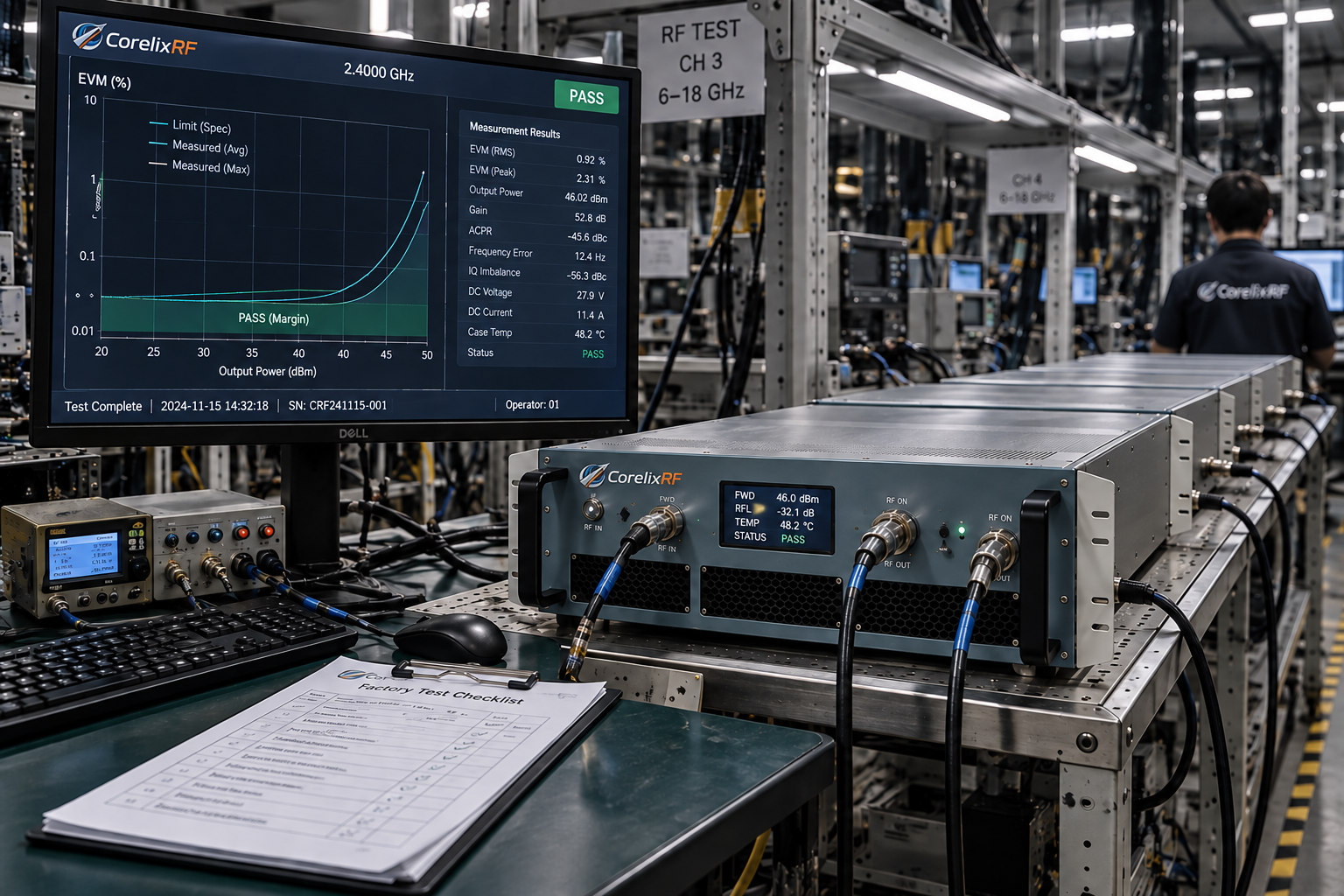
An EVM vs output power curve identifies the output range where an RF power amplifier preserves modulation quality with usable margin. At low power, noise and test-system limits often dominate; near compression, nonlinear distortion usually drives EVM upward. A project team that approves only the lowest point on the curve can miss thermal drift, unit spread, and waveform dependence. This guide explains how to run the sweep, read its regions, and select a defensible operating point for an RF power amplifier platform.
Throughout this article, any CorelixRF technical-documentation support, application review, customization path, or test-data recommendation is subject to project review, the supplied product configuration, and the project’s requirements.
Why Does EVM Change as Output Power Changes?
EVM changes because the balance between noise, phase error, and nonlinear distortion shifts as signal level rises. The familiar curve often falls, reaches a useful minimum region, and then rises, but its exact shape depends on the waveform and complete signal chain.
The Noise-Limited Region
At low output power, the desired signal approaches the combined noise and residual-error floor of the generator, amplifier, analyzer, and interconnections. Raising the level improves signal-to-noise ratio, so the measured EVM can improve even though the amplifier itself has not become more linear. Leakage, phase noise, and quantization effects may also become visible here.
The Compression-Limited Region
As drive increases, gain compression, AM-AM error, AM-PM conversion, clipping, and memory effects distort the modulation. The result may be a steep rise or a gradual shoulder. A change in current, gain, or spectrum at the same point helps confirm that the curve reflects the DUT rather than the analyzer.
| Power Region | Likely Dominant Limitation | Useful Follow-Up |
|---|---|---|
| Low level | Noise or residual instrument EVM | Measure the system floor and improve range |
| Middle region | Combined minimum impairments | Check width and repeatability |
| High level | Compression and memory effects | Review gain, ACLR, current, and temperature |
The table shows why the minimum point alone cannot explain the cause or define a production setting.
Key Takeaway: Read the curve as three operating regions, then verify the dominant impairment in each region.
Which Power Value Belongs on the Horizontal Axis?
Use average output power at a clearly named DUT reference plane unless the project requires a different definition. Input power, peak envelope power, and output backoff answer different questions and must not be silently substituted.
Average, Peak, and Backoff Values
Average RF output power supports thermal and transmitter-budget decisions. Peak envelope power describes the waveform peaks that approach instantaneous compression. Output backoff relates the chosen average level to a stated reference such as saturated power or a defined compression point, so the reference and measurement method must accompany the number.
Correct the Reference Plane
Account for cable, coupler, attenuator, adapter, and fixture loss between the amplifier connector and the measuring instrument. Apply frequency-dependent corrections once, and document their signs. The power amplifier test setup should make the output reference plane visible to every reviewer.
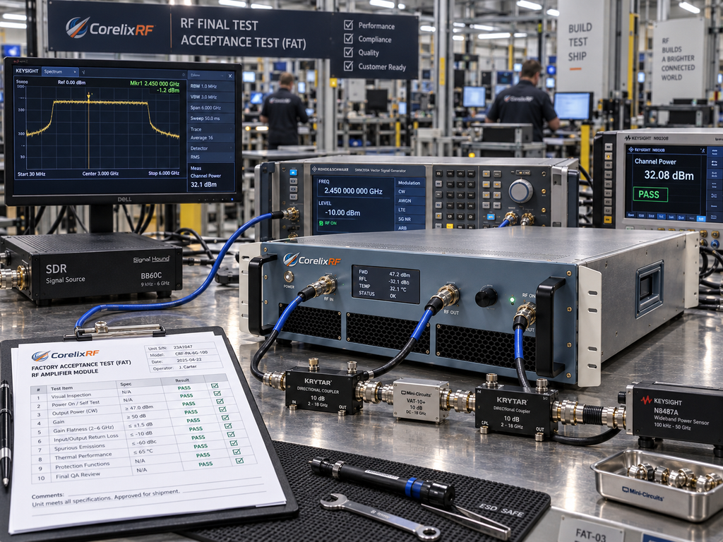
Key Takeaway: Label both the power quantity and the physical plane so another lab can reproduce the x-axis.
Which Signal Conditions Must Stay Fixed?
Keep the waveform, bandwidth, allocation, crest factor, filtering, sample rate, and correction state fixed throughout the sweep. A changed waveform can create a new curve even when the amplifier is unchanged.
Preserve Waveform Statistics
Record the modulation family, occupied bandwidth, resource allocation, subcarrier spacing where applicable, frame pattern, and peak-to-average power ratio. Use the same waveform file or an independently verified equivalent. If crest factor reduction is enabled, preserve its algorithm, settings, and resulting PAPR.
Record Linearization and Equalization
State whether digital predistortion, equalization, gain correction, or any transmitter calibration is active. Analyzer equalization and reference-signal processing can also change the result. When a project uses a custom SDR waveform chain, define which functions belong to the source and which belong to the amplifier test.
Key Takeaway: Treat the waveform configuration as part of the test article, not as an interchangeable stimulus.
How Do You Establish the Measurement Floor?
Measure the source-and-analyzer residual EVM across the intended level range before trusting DUT data. The floor must be comfortably better than the performance you want to distinguish.
Make a Through Measurement
Connect the source to the analyzer through a safe, calibrated path and use the same waveform, frequency, bandwidth, filtering, and analysis settings planned for the DUT. Sweep the received level or insert known attenuation. This reveals where receiver noise, source quality, or range switching changes the residual result.
Confirm Receiver Headroom
Adjust reference level and attenuation while holding the corrected input constant. A valid result should remain reasonably consistent; a large change suggests overload, insufficient range, or an analysis configuration problem. Include the analyzer’s residual EVM and uncertainty in the report rather than subtracting it as a simple scalar.
Key Takeaway: Demonstrate the test-system floor over the same received-power range used for the amplifier sweep.
How Should the RF PA Power Sweep Be Run?
Run a controlled, monotonic sweep with defined warm-up, step size, dwell, averaging, and repeat direction. Monitor electrical and thermal state at every step.
Start Below the Expected Working Region
Stabilize the amplifier with the specified supply, load, cooling, and baseplate or inlet condition. Begin at a low drive level, verify output and current, then advance in steps small enough to resolve the minimum region and compression knee. The input-drive and overdrive guide provides a practical framework for safe level control.
Repeat and Reverse the Sweep
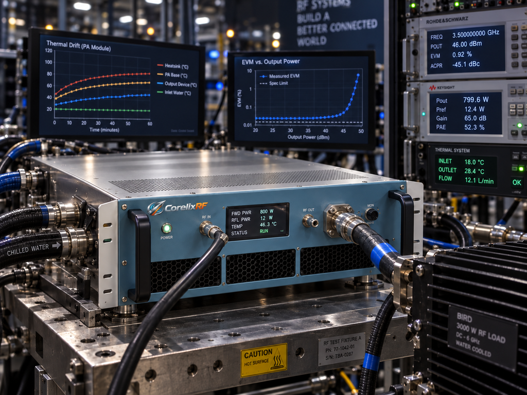
Use a consistent dwell time and enough analyzed frames to reduce random variation. Repeat the sweep and, where heating could matter, return from high to low power. Hysteresis between directions can reveal thermal memory, protection activity, gain-state changes, or insufficient stabilization.
Preserve Point-by-Point Data
Store numerical output power, EVM, gain, current, temperature, and instrument state for every step instead of relying on a rendered graph. Raw records allow a reviewer to recompute threshold crossings, compare repeated sweeps, and identify a range change hidden by line smoothing. Time stamps also help relate long sweeps to warm-up or drift.
| Sweep Field | What to Record | Why It Matters |
|---|---|---|
| Step and dwell | Actual power increment and time | Controls resolution and thermal state |
| Averaging | Frames, bursts, or symbols | Sets repeatability and comparability |
| Direction | Up, down, and repeat count | Reveals hysteresis and drift |
| Monitors | Gain, current, temperature, alarms | Connects EVM changes to DUT behavior |
The table converts a visual curve into a repeatable test sequence.
Key Takeaway: A useful sweep includes state monitoring and repeat data, not only an exported EVM trace.
How Do You Read EVM vs Output Power Data?
Find the threshold crossings and the width of the compliant region, then identify where the curve has adequate slope and margin. A broad, repeatable window is usually safer than a single impressive minimum.
Mark Limits and Curve Features
Overlay the applicable EVM limit and identify lower- and upper-power crossings. Note the minimum, flat region, sharp shoulders, discontinuities, and changes in scatter. The curve should be reviewed together with gain, output spectrum, current, and temperature collected at the same points.
Prefer an Operating Window
Define a candidate range that remains below the limit after measurement uncertainty and project margin are applied. Avoid choosing the exact threshold or absolute minimum. With EVM vs output power data, the distance to both the low-power floor and high-power compression region matters more than a single decimal place.
Key Takeaway: Approve a stable power window with margin on both sides instead of chasing the lowest plotted value.
How Do You Select the PA Operating Point?
Choose the lowest-risk point that meets output, modulation, efficiency, and thermal requirements across expected variation. The decision should include unit spread and environmental change rather than rely on the nominal curve.
Build the Margin Budget
Start with the applicable system or standard limit, then reserve margin for measurement uncertainty, temperature, supply tolerance, frequency, waveform variation, production spread, and aging where relevant. Avoid inventing a universal margin; assign each contribution from project evidence. Document which effects were measured and which remain engineering allowances.
Compare the Full Trade Space
At each candidate point, review EVM, average and peak output, gain, efficiency, ACLR, current, and heat load. An extra fraction of a decibel of output may consume substantial linearity or thermal margin. CorelixRF’s amplifiers by output power can narrow the hardware range, but test data must establish the modulated working point.
Key Takeaway: Select the operating point from a documented margin budget and several linked performance metrics.
What Can an Abnormal Curve Reveal?
An irregular curve can reveal a test artifact, mode transition, protection event, memory effect, or unstable operating condition. Diagnose the shape before treating it as normal amplifier behavior.
Diagnose Low- and Mid-Power Anomalies
A high or ragged low-power region can come from receiver noise, source residual EVM, synchronization failures, leakage, or range changes. A step in the middle may indicate an attenuator change, gain-state switch, calibration boundary, or control-loop transition. Repeat the point with fixed range settings and inspect constellation, spectrum, and time-domain views.
Diagnose High-Power Anomalies
Sudden degradation near the top of the sweep may indicate hard clipping, supply current limiting, thermal protection, bias movement, or analyzer overload. Hold selected points long enough to observe time dependence and compare with a thermal stability test method. Stop if electrical or thermal limits are approached.
Key Takeaway: Use synchronized electrical, spectral, and thermal evidence to explain every discontinuity in the curve.
How Can Two Amplifiers Be Compared Fairly?
Compare them with the same signal, reference plane, fixture, calibration, environment, and processing. Present both equal-output-power and equal-backoff views when they support different system decisions.
Control the Bench and Conditions
Use identical cables and losses where practical, or apply validated corrections. Match frequency, waveform, supply, load, cooling, temperature, averaging, and analyzer configuration. If each unit needs a different driver or attenuator, verify that those changes do not alter the measurement floor.
Normalize the Decision, Not the Evidence
Equal output power shows which device provides better modulation quality at the system’s required level. Equal backoff helps compare nonlinear behavior relative to a defined device limit. Preserve original measured curves and state every normalization so the comparison can be audited.
| Comparison View | Best Use | Main Caution |
|---|---|---|
| Equal average output | System working-point choice | Devices may have different rated capability |
| Equal output backoff | Relative linearity behavior | Backoff reference must match |
| Equal DC power or heat | Platform trade study | Does not replace output compliance |
The right comparison view follows the system decision rather than convenience.
Key Takeaway: Match the conditions first, then choose the comparison view that answers the actual procurement question.
What Should the Final Report Contain?
The report should contain raw and corrected curves, complete test conditions, the floor check, uncertainty, repeatability, and the proposed working point. It should also identify untested combinations.
Include Reproducible Evidence
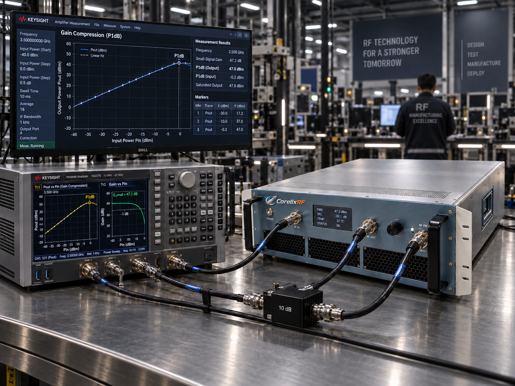
Record DUT identity and revision, waveform file or definition, frequency, bandwidth, PAPR, supply, bias, load, cooling, temperature, reference plane, path corrections, instrument states, dwell, averaging, and sweep direction. Add gain, current, spectrum, and thermal traces where they explain the curve. The test data a technical buyer should request provides a broader evidence checklist.
State the Approval Rule
Name the EVM limit and normalization, required output range, margin method, and pass/fail treatment of uncertainty. Mark the approved operating range and any conditions requiring retest. A buyer should be able to see whether the selected point is based on a typical unit, a guaranteed limit, or a production acceptance result.
Key Takeaway: Make the operating-point decision traceable to conditions, margin, and repeat evidence.
Conclusion
Reliable EVM vs output power testing separates the system floor, usable region, and compression behavior under one controlled waveform and reference plane. The final decision should use threshold crossings, window width, repeatability, margin, and related metrics rather than the minimum EVM alone. CorelixRF provides RF amplifier platforms and technical documentation that can support a model-level review. For a project with defined band, waveform, output target, cooling, and evidence requirements, contact the CorelixRF RF engineering team to discuss an appropriate test-data scope. Our engineering position is that a useful working point must remain defensible when the real operating conditions change.
FAQs
Why Does EVM Worsen at Very Low Output Power?
The desired signal becomes small relative to noise, leakage, phase noise, and residual test-system error. The measured value can therefore be limited by the source or analyzer before the amplifier becomes the dominant contributor. A through measurement across received power is the fastest way to identify this region.
Why Does EVM Rise Near Compression?
Near compression, amplitude and phase no longer follow the input linearly. Peaks may clip, and electrical or thermal memory can spread errors across the waveform. Confirm the cause by reviewing gain, spectrum, current, and temperature at the same power points.
Should the Curve Use Input or Output Power?
Average output power at the DUT plane is usually most useful for system selection, but input power can help diagnose gain behavior. The report may show both if each axis is defined and calibrated. Never compare curves that silently use different quantities.
How Much EVM Margin Should a Design Retain?
There is no universal value. Build the margin from measurement uncertainty, temperature, frequency, supply, waveform, unit spread, and any specified life condition. A project-specific budget is more defensible than a fixed rule of thumb.
Can Curves with Different Waveforms Be Compared?
Only as separate operating cases. Different bandwidth, allocation, PAPR, filtering, or predistortion can change PA stress and analyzer processing. For a direct device comparison, hold those waveform characteristics constant.