
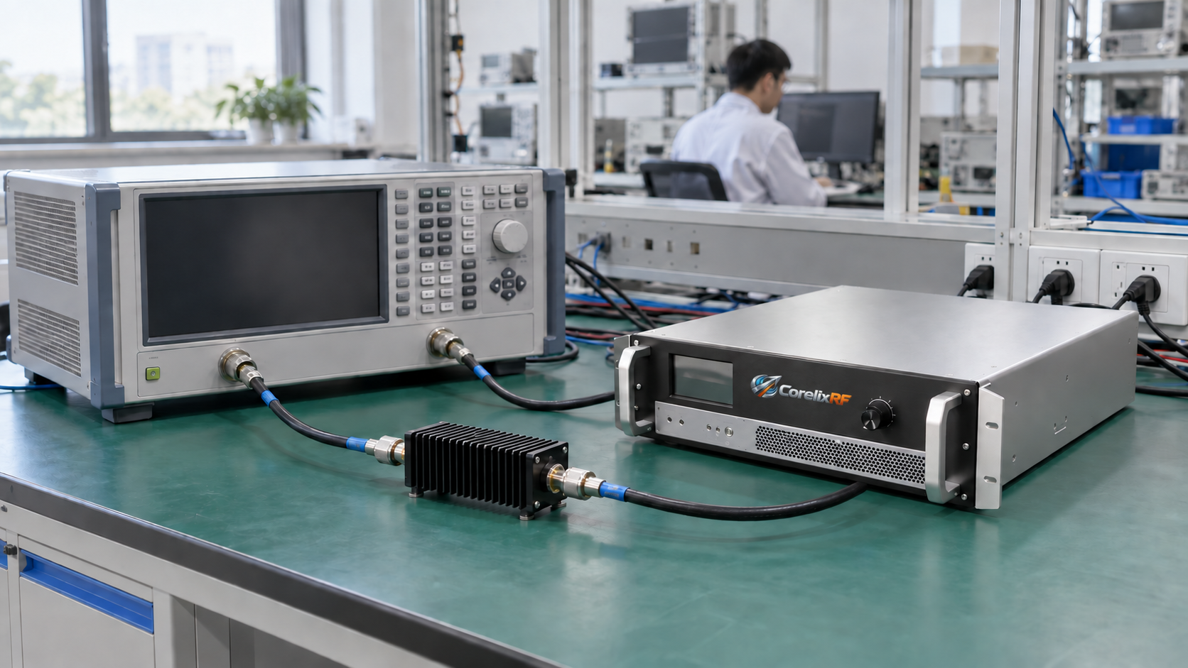
S-parameters measurement on an active RF amplifier requires a defined operating state, calibrated reference planes and a verified power budget. A low VNA source setting can still produce excessive receiver input after amplification. These seven steps cover setup, acquisition and repeatability, followed by a data-handoff checklist. The numerical example is a planning exercise, not a measured result or a universal instrument preset.
- Define quantities and acceptance conditions
- Budget forward and reverse power
- Calibrate the complete measurement paths
- Stabilize bias and verify small-signal operation
- Select and check sweep settings
- Acquire all four complex S-parameters
- Check repeatability and uncertainty
1. Define the S-Parameters and Acceptance Conditions
For a two-port network, each S-parameter relates an outgoing wave to an incident wave while the other port has zero incident wave. All four quantities contain magnitude and phase. Record port order and reference impedance before measuring; a reversed port assignment changes how downstream engineers interpret an S2P file.
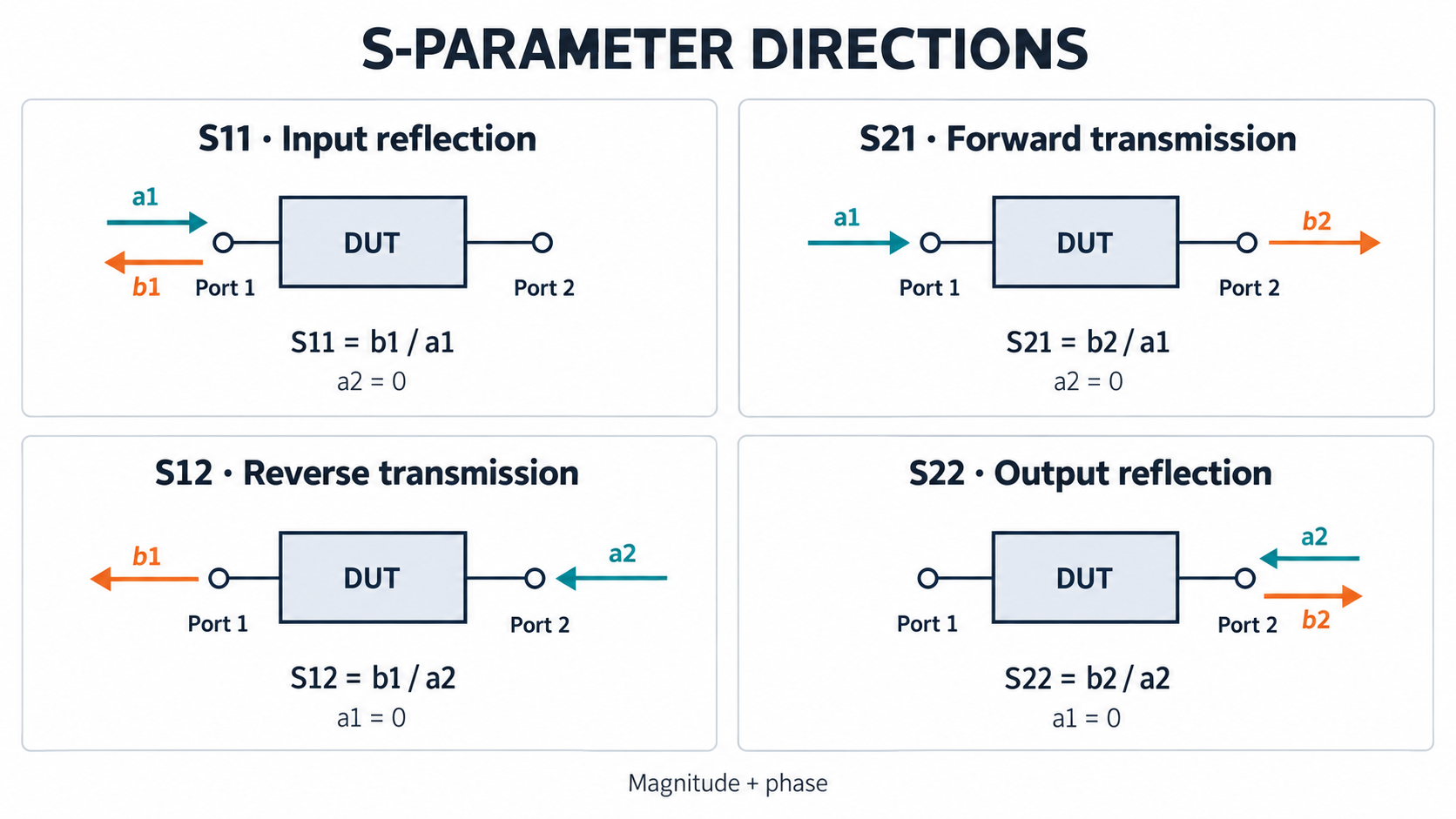
| Parameter | Meaning | Use |
|---|---|---|
| S11 | Input reflection | Input matching and source interaction |
| S21 | Forward transmission | Small-signal transmission gain and phase |
| S12 | Reverse transmission | Reverse coupling and stability calculations |
| S22 | Output reflection | Output matching and load interaction |
Define frequency range, bias, temperature, gain-control state and acceptance criteria together. Compare S21 against a gain specification only when its stated drive and operating conditions match your measurement. Magnitude-only plots cannot replace complex data for matching or stability calculations.
What the 1–2 GHz Product Example Establishes
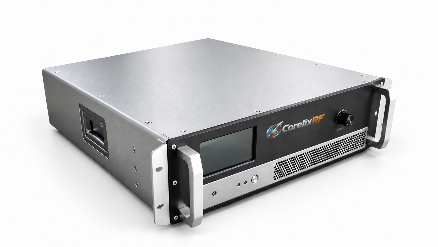
The CorelixRF CRF-PA-1000M2000M-50W datasheet lists 1–2 GHz coverage, 50 W rated output, 47 dB minimum gain and ±3 dB gain flatness. It also specifies 50 Ω input impedance, 1.5:1 maximum input VSWR, 5 dBm maximum input and SMA-female RF connectors. These are product specifications, not a complete small-signal measurement record.
At a VSWR limit of 1.5:1, |Γ| ≤ (1.5 − 1)/(1.5 + 1) = 0.20. The corresponding return loss is at least 13.98 dB, or S11 log magnitude no higher than −13.98 dB, under applicable specification conditions. This conversion does not establish measured phase or performance at other bias and drive states.
Use the UHF amplifier family page for platform selection. For specification review, request the exact model datasheet, revision and test conditions through the datasheet access page. A family page does not replace a model-specific source.
2. Budget Forward and Reverse Power Before Enabling the DUT
Draw every RF path, including cables, attenuators, couplers, bias tees, switches and terminations. Check each component across frequency and for every source direction. Follow specified bias sequencing, current limits and cooling requirements before applying RF.
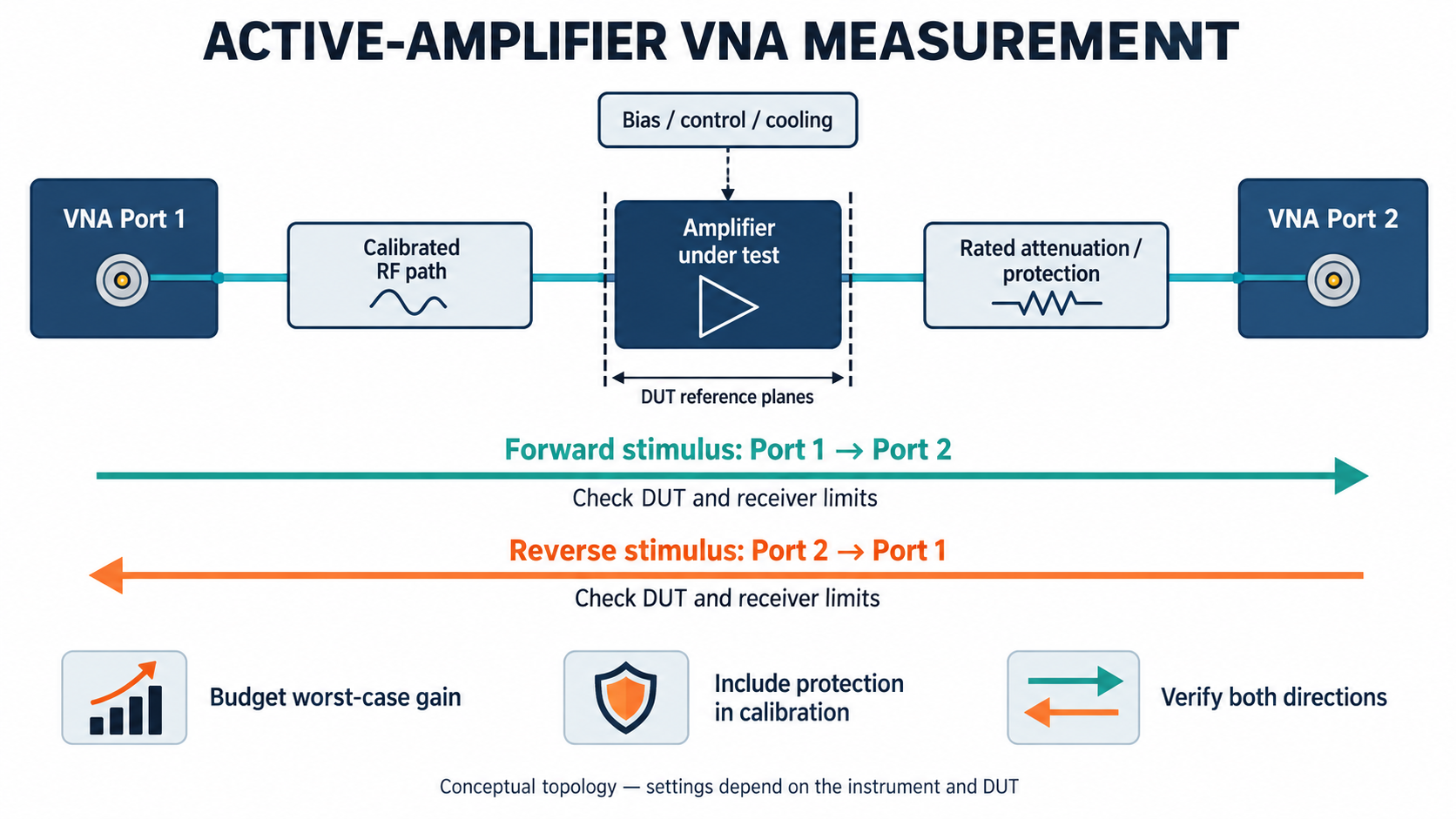
For a linear forward-path estimate, PRX ≈ PIN,DUT + G − A, with powers in dBm and gain or attenuation in dB. Use an upper bound for gain and a lower bound for path attenuation. Include source-level uncertainty, mismatch and operating-state variation. A minimum gain specification, such as 47 dB, cannot establish a safe upper power bound.
Check receiver compression and hardware damage limits separately. Internal receiver attenuation may not protect every component ahead of that attenuator. Keysight’s output-power measurement guidance distinguishes inaccurate measurements caused by compression from physical receiver damage.
Worked Example with Assumed Values
The following assumptions describe a hypothetical chain. They are not verified limits or recommended settings for the CorelixRF model or any particular VNA.
| Quantity | Assumed value | Role in the calculation |
|---|---|---|
| DUT input power | −40 dBm | At the calibrated DUT input plane |
| Maximum small-signal gain | 50 dB | An assumed upper bound, not the 47 dB minimum specification |
| Minimum output-path attenuation | 30 dB | Including frequency variation and tolerance |
| Allowed receiver input | −10 dBm | An assumed linear-measurement ceiling |
| Required margin | 6 dB | An assumed engineering allowance |
Estimated DUT output is −40 + 50 = +10 dBm. Estimated receiver input is +10 − 30 = −20 dBm, giving 10 dB below the assumed ceiling. With a 6 dB allowance, this simplified calculation permits PIN,DUT ≤ −10 + 30 − 50 − 6 = −36 dBm. It does not verify small-signal behavior or fault protection.
Check a different operating state separately. If 50 W reached this path, its approximately +47 dBm output would become +17 dBm after 30 dB attenuation. That exceeds the example’s receiver ceiling. A nominal low-drive calculation cannot cover unintended high output, oscillation or switching transients. Rated power is not necessarily a worst-case upper bound either.
Select attenuation, sampling, load ratings and any interlocks from verified maximum levels before enabling the amplifier. Confirm permissible reverse injection at its output port and VSWR protection behavior. The initial sweep must operate inside an already checked envelope.
3. Calibrate the Complete Measurement Paths
Place reference planes where the data user expects them. Include protection networks in calibration or apply a validated correction that accounts for their complex response. Scalar loss compensation alone does not remove phase delay or mismatch errors.
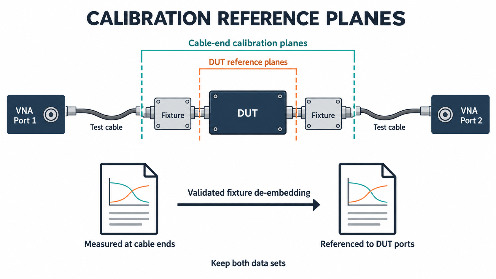
SOLT uses short, open, load and thru standards and often suits coaxial connections. TRL calibration uses thru, reflect and line standards and can suit fixtures, waveguides or on-wafer measurements. Its usable band and reference impedance depend on those standards. Electronic calibration also requires correct connector definitions and verification.
- Inspect connectors, use specified torque and support cables before calibration.
- Select compatible standards and record kit identification, frequency range and instrument settings.
- Calibrate with the measurement paths and attenuation configuration intended for acquisition.
- Measure an independent check device at the intended reference planes and save its comparison trace.
Changing cables, fixtures or attenuator states can invalidate correction. Follow the instrument’s requirements for recalibration or validated state-specific corrections. De-embed fixtures only with a checked model; retain both original and de-embedded data. A characterized thru or alternate fixture can help reveal model errors.
4. Stabilize Bias and Verify Small-Signal Operation
Record supply voltage, idle current, enable state, gain setting, temperature sensor location and warm-up conditions. Maintain the specified cooling conditions. Unexpected current changes or protection events require investigation before accepting traces.
Choose initial drive using verified gain and power limits, with enough headroom below compression across frequency. The product’s 5 dBm maximum input rating does not define a suitable VNA stimulus. Confirm delivered power at the DUT plane rather than assuming it equals the source display.
After checking the setup, acquire one sweep and repeat at a lower drive while maintaining valid calibration and receiver operation. In the hypothetical example, −40 and −45 dBm would give a 5 dB comparison. These levels are illustrative and require verification for an actual DUT.
Compare complex S21 and reflection data against an acceptance band derived from measurement uncertainty and project requirements. A change can indicate DUT nonlinearity, receiver compression, range switching or poor signal-to-noise ratio. Lowering drive indefinitely can make weak terms unusable; investigate the cause rather than accepting either trace by default.
5. Select Sweep Settings and Check Their Effect
Point spacing must resolve relevant features. IF bandwidth, averaging and dwell determine noise, settling and acquisition time. Choose settings while checking that longer measurements do not shift amplifier temperature or control state.
| Setting | Illustrative starting value | Verification needed |
|---|---|---|
| Span and points | 1–2 GHz, 401 linear points | 2.5 MHz spacing may miss narrow resonances; increase density where needed |
| IF bandwidth | 1 kHz | Check weak-term noise and sweep duration |
| Averaging | 4 sweeps | Keep individual sweeps to detect drift |
| Added dwell | 10 ms per point | Compare with a longer dwell; this may be insufficient for some controls |
These values are an example of documenting settings, not a qualified recipe. Actual frequency coverage, timing and receiver options come from the DUT and VNA. Repeat a representative sweep with finer spacing, narrower IF bandwidth or longer dwell, changing one variable at a time. Keep settings that resolve the required behavior without hiding time variation.
6. Acquire All Four Complex S-Parameters
Verify forward S11 and S21 measurements before enabling reverse acquisition. For S12 and S22, check injected power at the DUT output, reverse-path attenuation and receiver range. Both directions need an appropriate linear stimulus and enough dynamic range.
Handle High Gain and Weak Reverse Signals
A high-gain amplifier may need very low forward drive. Applying that same source level in reverse can leave S12 or S22 dominated by noise, especially behind output attenuation. In a full two-port correction, noisy reverse measurements can also affect corrected forward results.
Where supported, set port powers independently and follow the instrument-specific calibration procedure. Keysight’s high-gain amplifier measurement guide explains this tradeoff. Enhanced response calibration can suit some forward-only measurements, but it does not supply equivalent correction for S12 and S22 or replace a complete two-port dataset.
Save magnitude and phase for all four terms with a consistent port map. Flag points near the usable noise floor. A smooth-looking trace below adequate signal-to-noise ratio cannot establish reverse isolation. Retain unprocessed data while investigating spikes, discontinuities or receiver range changes.
7. Check Repeatability and State Measurement Limits
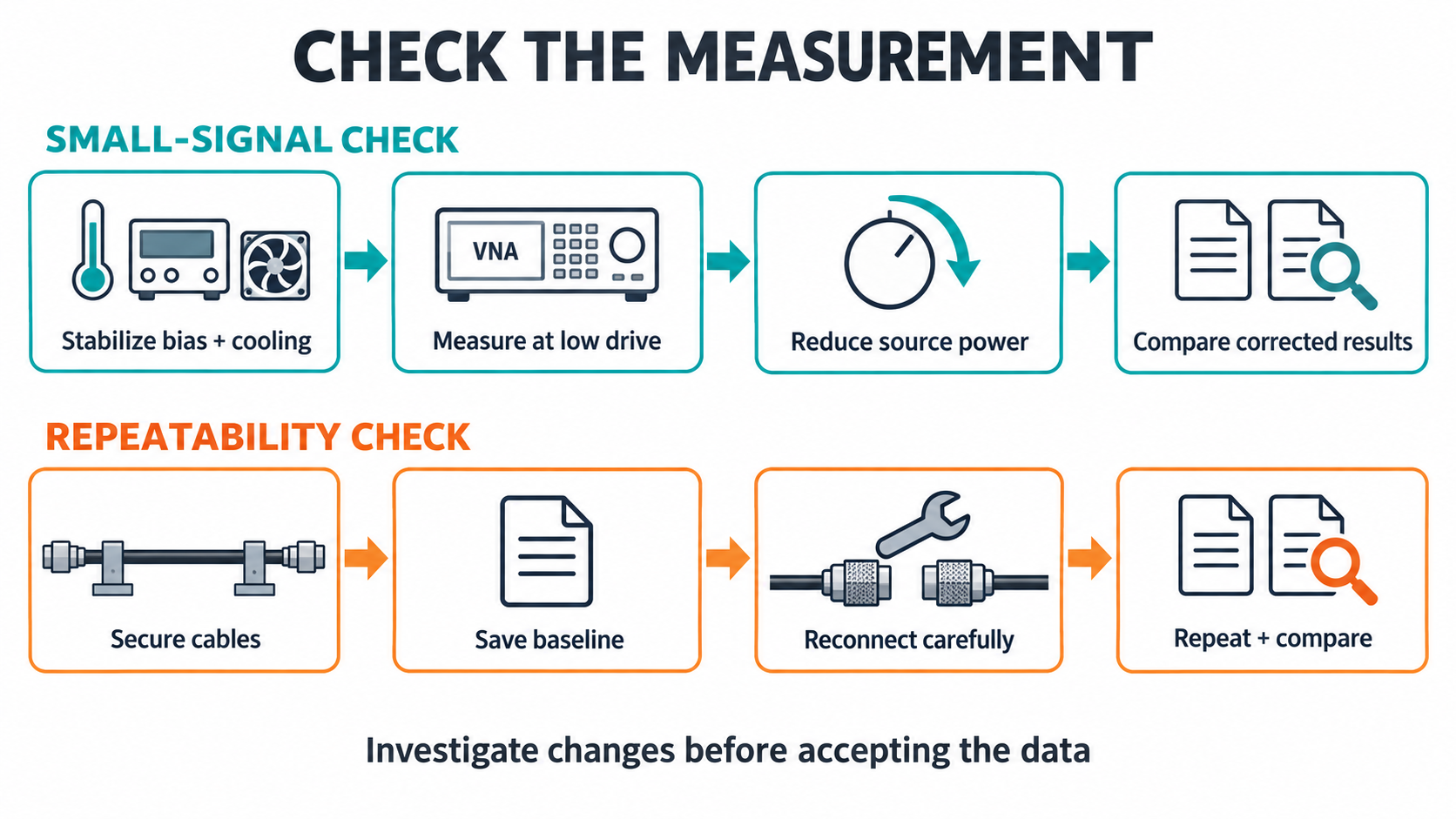
Repeat an unchanged sweep to characterize short-term variation. Then perform a controlled reconnection and repeat the measurement with consistent torque and cable routing. Revisit the check device after a long run or suspected drift. Recalibrate when the validated setup conditions no longer apply.
- Compare repeated complex traces across frequency, including band edges and narrow features.
- Record maximum gain and phase differences; align phase wrapping before comparison.
- Separate unchanged-setup variation, reconnection spread and recalibration differences.
- Identify noise-floor, overload and missing-data regions without smoothing them away.
Set acceptance limits before reviewing results, based on measurement capability and the intended engineering decision. Repeatability alone is not a complete uncertainty budget: a stable calibration error can remain across repeated sweeps.
NIST’s study of VNA receiver nonlinearities discusses receiver effects alongside noise, drift and cable position. Its experiment covers WR-15 waveguide measurements; its numerical results should not be transferred directly to a 1–2 GHz coaxial setup.
Deliver the S2P File with Its Conditions and Limits
A Touchstone file needs enough accompanying information for another engineer to interpret and reuse it. Organize the package with the test and delivery documentation, including the following records.
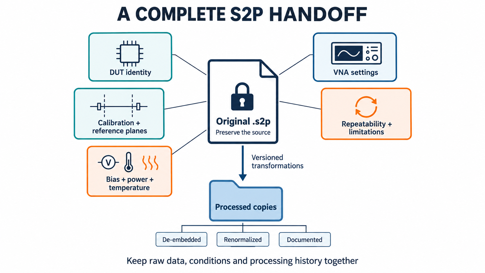
| Record | Required information |
|---|---|
| DUT and state | Model, serial number, revision, supply, bias, temperature, control state and cooling |
| Measurement | Instrument configuration, calibration, reference planes, source levels in both directions and sweep settings |
| Data interpretation | Port order, frequency units, reference impedance, complex format and any transformations |
| Evidence and release | Original S2P, setup file, check-device results, repeat traces, limits, exceptions, date and reviewer |
Keep original files unchanged and version every de-embedded, renormalized or converted derivative. A short README should identify source files, processing software and transformations. Check representative frequencies after conversion to catch port swaps, unit errors or altered phase conventions.
Where Small-Signal Data Stops Answering the Question
Complete S-parameters can predict linear mismatch effects when combined with source and load reflection coefficients, provided the modeled operating state remains valid and stable. The Genesys simulation manual’s matching discussion describes this use of two-port data.
Compression, saturated output, distortion, protection switching and driven output match need measurements or models appropriate to those operating states. A small-signal S2P file does not prove rated-power performance under mismatched loads. Use power, gain and thermal testing alongside the technical buyer’s test-data checklist when specifying acceptance evidence.
For a model-specific review, send CorelixRF your required frequency band, operating state, reference planes and data format. Identify whether you need small-signal S-parameters or powered performance so available evidence and any additional testing can be discussed.
FAQs
How Low Should VNA Source Power Be?
Use verified maximum gain, delivered DUT power and receiver limits to establish a starting range. Confirm linear operation through a lower-drive comparison without losing adequate signal-to-noise ratio. There is no source setting that suits every amplifier.
Why Can an Amplifier Damage a VNA Receiver?
Amplification, switching transients or oscillation can exceed receiver and test-port ratings. Calculate every relevant path and install suitable protection before enabling the DUT. Receiver compression can cause errors below a damage threshold.
What Is the Difference between SOLT and TRL?
SOLT uses short, open, load and thru standards. TRL uses thru, reflect and line standards. Connector geometry, available standards, bandwidth and required uncertainty determine which method fits a setup.
Which Metadata Should Accompany an S2P File?
Include DUT identity, port order, reference impedance, calibration planes, bias, temperature and source levels for both directions. Attach sweep settings, correction details, repeatability evidence and any limitations on reuse.
Can Small-Signal Data Predict Saturated PA Performance?
Small-signal data characterize a linearized response around a stated operating point. Saturated output, efficiency, distortion and large-signal mismatch behavior require suitable powered measurements or validated nonlinear models.